LSTM is a type of recurrent neural network that is widely used in natural language processing, speech recognition, and other applications where sequential data is important. LSTMs are particularly effective at capturing long-term dependencies in sequences of data, which can be challenging for other types of neural networks.
Navigating the jargon associated with the components of LSTM networks can be daunting, even for those familiar with neural networks. Terms like “cell,” “layer,” “unit,” and “neuron” are often thrown around without a clear explanation of their meaning and purpose. However, understanding these components is crucial for building and fine-tuning LSTM models. So what exactly are these terms, and how do they benefit the network?
🌟 “unit” = “neuron”
🌟 “cell” = a collection of “neurons”
🌟 “layer” = a stack of “cells”
An LSTM Neuron
The colah blog shows the core idea behind LSTMs, nicely illustrating the 4 gates inside an LSTM neuron.
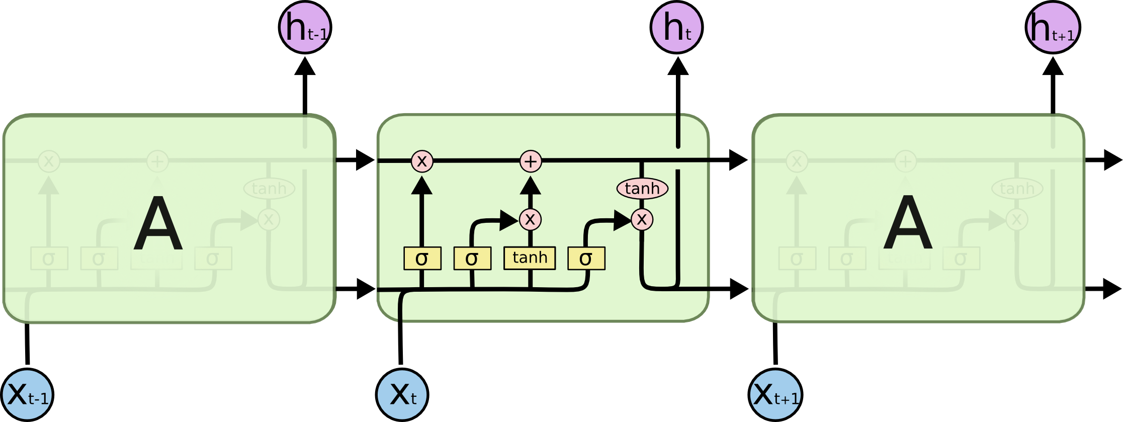
Fig. 1. LSTM neuron. (Image source: colah blog)
The number of units defines the dimension of the hidden states, which is the same as that of the cell state.
Let $h$ denote the length of hidden states – the number of hidden units, which is called hidden_size in PyTorch and num_units in Tensorflow.
An LSTM Cell
Here is an example LSTM cell that contains $h=2$ LSTM neurons.
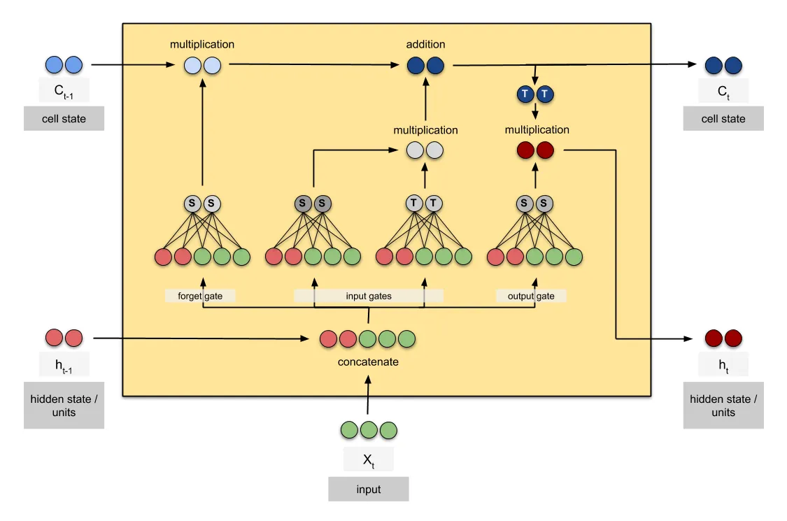
Fig. 2. LSTM cell. (Image source: Raimi Karim)
The 4 gates in an LSTM neuron suggest that an LSTM neuron has 4 feed-forward neural networks. If we have a sample input of feature size $i$ (e.g., $i=3$ in Fig. 2), we concatenate the sample input with the hidden state and then pass them ($i+h$) together to the gates. The number of parameters in this LSTM cell can be calculated as: $$ 4 \times [h(h+i) + h] $$
The “layer” is a collection of cells that are stacked on top of each other to form the architecture of the network.
So take on the challenge and unlock the full potential of LSTMs!