Risk-sensitive Distributional Reinforcement Learning

Reinforcement learning (RL) is a powerful framework for training agents to maximize cumulative reward, but it typically assumes risk-neutrality. This can lead to suboptimal behavior in practical scenarios where the consequences of unfavorable outcomes can be detrimental.

What is risk?

Generally, risk might arise whenever there is uncertainty. In a financial situation, investment risk can be identified with uncertain monetary loss. In a safety-critical engineering system, risk is the undesirable detrimental outcome.

How do we measure risk?

Risk metrics typically involve probability distribution of outcomes and quantified loss for each outcome.

The standard deviation is a measure of uncertainty, but not a good choice for risk measure. Risk concerns only losses, but standard deviation can’t account for such asymmetric nature.

Artzner et. al. (1998) provided an axiomatic definition that a risk measure should satisfy, which is called coherent risk measure. They denote the risk measure by the functional $\rho(X)$, which assigns a real-valued number to a random variable $X$. $X$ can be thought of as payoffs or returns.

Monotonicity: $\rho(Y) \leq \rho(X)$ if $Y \geq X$.
Positive Homogeneity: $\rho(0) = 0, \rho(\lambda X) = \lambda \rho(X)$ for all $X$ and all $\lambda > 0$.
Sub-additivity: $\rho(X+Y) \leq \rho(X) + \rho(Y)$ for all $X$ and $Y$.
Translation invariance: $\rho(X+Y) = \rho(X) -C$ for all $X$ and $C \in \mathbb{R}$.

The positive Homogeneity and sub-additivity imply that the functional is convex, $$ \rho(\lambda X+ (1-\lambda)Y) \leq \rho(\lambda X) + \rho((1-\lambda)Y) = \lambda \rho(X) + (1-\lambda) \rho(Y) $$ where $\lambda \in [0,1]$. This convexity property supports the diversification effect: The risk of a portfolio is no greater than the sum of the risks of its constituents.

The translation invariance shows the minimum amount of capital requirements to hedge the risk $\rho(X)$, $\rho(X+\rho(X)) = 0$.

A commonly used coherent risk measure is the expected shortfall, also known as the conditional value at risk, i.e., CVaR. See also other risk measures: Value at risk (VaR), Entropic value at risk (EVaR), etc.

Risk-sensitive distributional reinforcement learning

Quantiles

Let $Z$ be a continuous random variable with a probability density $f$, the cumulative distribution function $F$, and $\tau \in (0, 1)$, then the $τ$-th quantile of $Z$, $z_{\tau}$ is the inverse of its c.d.f. $$z_{\tau} = F^{-1}(\tau), \tau = F(z_{\tau}) = \int_{-\infty}^{z_{\tau}}f(z)\mathop{\mathrm{d}}z.$$ We have $$\tau = F(z), \mathop{\mathrm{d}}\tau = F'(z)\mathop{\mathrm{d}}z = f(z)\mathop{\mathrm{d}}z $$ $$ \int_0^1 F^{-1}(\tau)\mathop{\mathrm{d}}\tau = \int_{\infty}^{\infty}F^{-1}(F(z))F'(z)\mathop{\mathrm{d}}z = \int_{\infty}^{\infty} zf(z)\mathop{\mathrm{d}}z = \mathbb{E}(z) $$

Quantile Regression

sklearn.linear_model.QuantileRegressor is a method for estimating $F^{-1}(\tau)$

As a linear model, the QuantileRegressor gives linear predictions $\hat{z}(w, X) = Xw$ for the $\tau$-th quantile ($X:= (x,a)$). The weights $w$ are then found by the following minimization problem: $$\min_{w} {\frac{1}{n_{\text{samples}}} \sum_i PB_{\tau}(z_i - X_i w) + \alpha ||w||_1}. $$ The quantile regression loss (a.k.a pinball loss or linear loss) is

$$ PB_{\tau}(u) = |\tau - \mathbb{I}_{u \leq 0}|u = \tau \max(u, 0) + (1 - \tau) \max(-u, 0) = \begin{cases} \tau u, & u > 0, \\ 0, & u = 0, \\ (\tau-1) u, & u < 0 \end{cases} $$

Implicit Quantile Network

is a deterministic neural network parameterizes $(x, a, \tau)$ and output the quantile of the target distribution $z_{\tau} = F^{-1}(\tau) \approx Q_{\theta} (x, a; \tau)$

The IQN loss minimizes sampled errors for $Z$ at different $\tau$s:
1. Sample $\tau_i \sim U([0,1])$ for $N$ times, $i = 1, \dots, N$
2. $\mathcal{L}(x) = \frac{1}{N}\sum_i PB_{\tau_i}(z_{\tau_i} - Q_{\theta} (x, a; \tau_i))$ (If the entire target distribution $Z$ is not accessible, $z_{\tau_i}$ is replaced with a single target scalar z as an approximation.)
Instead of the PB loss, Dabney et al., 2018 used the Huber quantile regression loss with threshold $\kappa$:

$$ \rho_{\tau}^{\kappa}(u)= \begin{cases} |\tau - \mathbb{I}_{u \leq 0}|\frac{u^2}{2\kappa}, & |u| \leq \kappa, \\ |\tau - \mathbb{I}_{u \leq 0}|(|u|-\frac{1}{2}\kappa), & |u| > \kappa \end{cases} $$

Policy

The advantage of estimating $Z$ through randomly sampled $\tau$: Risk-sensitive policy.

Risk refers to the uncertainty over possible outcomes and risk-sensitive policies are those which depend upon more than the mean of the outcomes. Here, the uncertainty is captured by the distribution over returns. Let’s take a simple illustrative risk-sensitive criterion Javier Garćıa and Fernando Ferńandez, 2015: $$ \max_{\pi}(\mathbb{E}(z) - \beta \mathrm{Var}(z)) $$

Risk-neutral policy

$$ \pi(x) = \underset{a}{\arg\max} \mathbb{E}[z] = \frac{1}{N}\sum_i Q_{\theta}(x, a; \tau_i) $$

Risk-sensitive Policy

$$ {\pi}(x) = \underset{a}{\arg\max} \mathbb{E}[U(z)], $$ which is equivalent to maximizing a distorted expectation using a distortion risk measure for some continuous monotonic function $h$: $$ {\pi}(x) = \underset{a}{\arg\max} \int_{\infty}^{\infty} z \frac{\partial (h \circ F(z))}{\partial z} \mathop{\mathrm{d}}z. $$

Let $\beta : [0, 1] \rightarrow [0, 1]$ be a distortion risk measure.

$$ \begin{aligned} {\pi}(x) &= \underset{a}{\arg\max} \int_{0}^{1} F^{-1}(\tau) (\frac{\partial \beta}{\partial \tau} \circ F'(z)) \mathop{\mathrm{d}}z \\ &= \underset{a}{\arg\max} \int_{0}^{1} F^{-1}(\tau) \mathop{\mathrm{d}} \beta(\tau) \end{aligned} $$

$$ {\pi}(x) = \underset{a}{\arg\max} \frac{1}{N} \sum_i Q_{\theta}(x, a; \beta(\tau_i)) $$

Example of a risk-averse policy: CVaR (Chow & Ghavamzadeh, 2014)

$$ \mathrm{CVaR}(\eta, \tau) = \eta \tau $$ $$ ~{\pi}(x) = \underset{a}{\arg\max} \mathbb{E}[\eta z] $$

Evaluating under different distortion risk measures is equivalent to changing the sampling distribution for $\tau$ , allowing us to achieve various forms of risk-sensitive policies.

Implementation

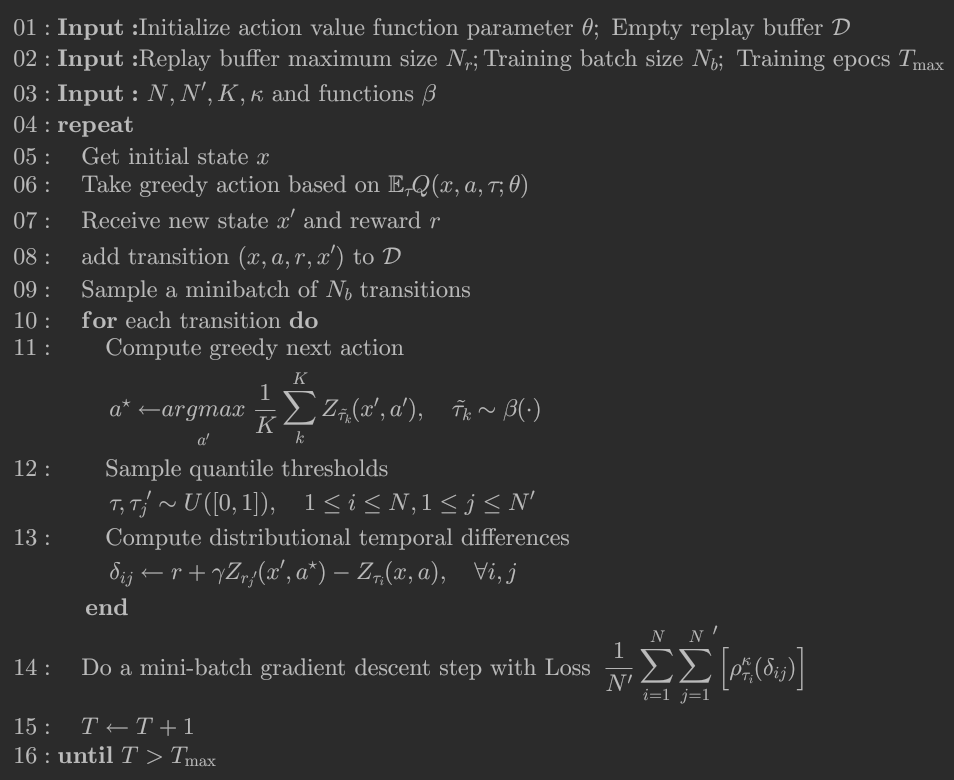
Architecture

Convolutional layers $\psi: \mathcal{X} \rightarrow \mathbb{R}^d$
Fuly-connected layers $f: \mathbb{R}^d \rightarrow \mathbb{R}^{|\mathcal{A}|}$
$Q(x,a) \approx f(\psi(x))_a$
Embedding for the sample $\tau$: $\phi(\tau): [0,1] \rightarrow \mathbb{R}^d$ $$\phi_j(\tau):= \mathrm{ReLU}(\sum_{i=0}^{n-1}\cos(\pi i \tau)w_{ij} + b_j)$$ i: hidden layer size of the embedding, e.g., $n = 64$

j: output size of the embedding, $d$
$Q(x,a; \tau) \approx f(\psi(x) \odot \phi(\tau))_a$

the encoding of $x$ and embedding for $\tau$ are flexible, which should be experimented.

Citation

Cited as:

Guo, Rong. (November 2022). Risk-sensitive Distributional Reinforcement Learning. Rong’Log. https://rongrg.github.io/posts/2022-11-11-riskrl/.

@article{guo2022riskRL,
  title   = "Risk-sensitive Distributional Reinforcement Learning",
  author  = "Guo, Rong",
  journal = "rongrg.github.io",
  year    = "2022",
  month   = "November",
  url     = "https://rongrg.github.io/posts/2022-11-11-riskrl//"
}

What is risk?#

How do we measure risk?#

Risk-sensitive distributional reinforcement learning#

Quantiles#

Quantile Regression#

Implicit Quantile Network#

Policy#

Risk-neutral policy#

Risk-sensitive Policy#

Example of a risk-averse policy: CVaR (Chow & Ghavamzadeh, 2014)#

Implementation#

Architecture#

Citation#

Reference#